Documentation Index
Fetch the complete documentation index at: https://nixtla.io/docs/llms.txt
Use this file to discover all available pages before exploring further.
What Are Quantile Forecasts?
Quantile forecasts correspond to specific percentiles of the forecast distribution and provide a more complete representation of the range of possible outcomes.- The 0.5 quantile (or 50th percentile) is the median forecast, meaning there is a 50% chance that the actual value will fall below or above this point.
- The 0.1 quantile (or 10th percentile) forecast represents a value that the actual observation is expected to fall below 10% of the time.
- The 0.9 quantile (or 90th percentile) forecast represents a value that the actual observation is expected to fall below 90% of the time.
Why Use Quantile Forecasts
- Quantile forecasts can provide information about best and worst-case scenarios, allowing you to make better decisions under uncertainty.
- In many real-world scenarios, being wrong in one direction is more costly than being wrong in the other. Quantile forecasts allow you to focus on the specific percentiles that matter most for your particular use case.
How to Generate Quantile Forecasts
Step 1: Import Packages
Import the required packages and initialize a Nixtla client to connect with TimeGPT.Step 2: Load Data
In this tutorial, we will use the Air Passengers dataset.| timestamp | value | |
|---|---|---|
| 0 | 1949-01-01 | 112 |
| 1 | 1949-02-01 | 118 |
| 2 | 1949-03-01 | 132 |
| 3 | 1949-04-01 | 129 |
| 4 | 1949-05-01 | 121 |
Step 3: Forecast with Quantiles
To specify the desired quantiles, you need to pass a list of quantiles to thequantiles parameter. Choose quantiles between 0 and 1 based on your uncertainty analysis needs.
| timestamp | TimeGPT | TimeGPT-q-10 | TimeGPT-q-20 | TimeGPT-q-30 | TimeGPT-q-40 | TimeGPT-q-50 | TimeGPT-q-60 | TimeGPT-q-70 | TimeGPT-q-80 | TimeGPT-q-90 |
|---|---|---|---|---|---|---|---|---|---|---|
| 1961-01-01 | 437.84 | 431.99 | 435.04 | 435.38 | 436.40 | 437.84 | 439.27 | 440.29 | 440.63 | 443.69 |
| 1961-02-01 | 426.06 | 412.70 | 414.83 | 416.04 | 421.72 | 426.06 | 430.41 | 436.08 | 437.29 | 439.42 |
| 1961-03-01 | 463.12 | 437.41 | 444.23 | 446.42 | 450.71 | 463.12 | 475.53 | 479.81 | 482.00 | 488.82 |
| 1961-04-01 | 478.24 | 448.72 | 455.43 | 465.57 | 469.88 | 478.24 | 486.61 | 490.92 | 501.06 | 507.76 |
| 1961-05-01 | 505.65 | 478.41 | 493.16 | 497.99 | 499.14 | 505.65 | 512.15 | 513.30 | 518.14 | 532.89 |
- Each requested quantile gets its own column named in the format
TimeGPT-q-... - The
TimeGPTcolumn shows the mean forecast - The mean forecast (
TimeGPT) is identical to the 0.5 quantile (TimeGPT-q-50)
Step 4: Plot the Quantile Forecasts
To plot the quantile forecasts, you can use theplot method.
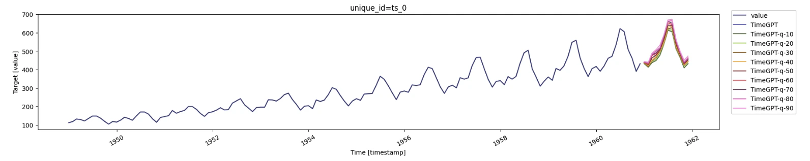
- The actual time series data in blue.
- Multiple forecast intervals represented by different quantiles:
- The 0.5 quantile (50th percentile) represents the median forecast.
- The 0.1 and 0.9 quantiles (10th and 90th percentiles) show the outer bounds of the forecast.
- Additional quantiles (0.2, 0.3, 0.4, 0.6, 0.7, 0.8) are shown in between, creating a gradient of uncertainty.
- Shows the full distribution of possible outcomes rather than just a single point forecast.
- Helps identify best and worst-case scenarios.
- Allows decision-makers to understand the range of uncertainty in the predictions.
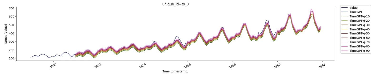
Step 5: Historical Forecast
You can also use quantile forecasts to forecast historical data by setting theadd_history parameter to True.
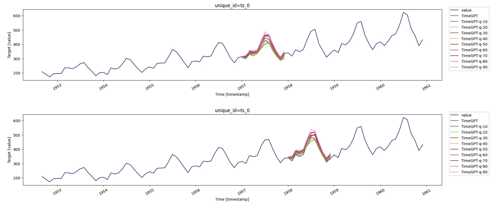
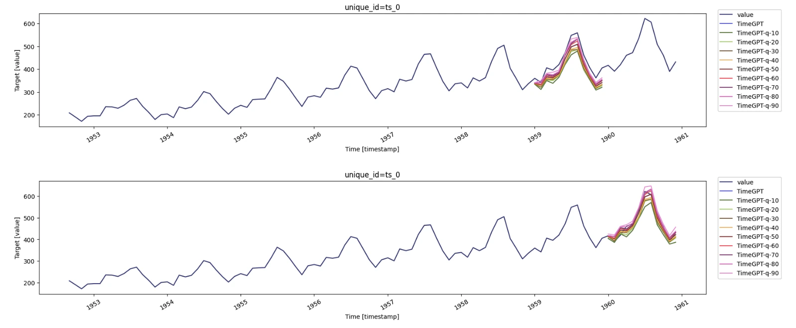
Step 6: Cross-Validation
To evaluate the performance of the quantile forecasts across multiple time windows, you can use thecross_validation method.
Congratulations! You have successfully generated quantile forecasts using TimeGPT. You also visualized historical quantile predictions and evaluated their performance through cross-validation.